Optimizing the Collaboration Structure in Cross-Silo Federated Learning
Wenxuan Bao1, Haohan Wang1, Jun Wu1, Jingrui He1
1University of Illinois Urbana-Champaign
ICML 2023 [arxiv] [poster] [slides] [talk] [code] [virtual site (registration required)]
Paper Summary
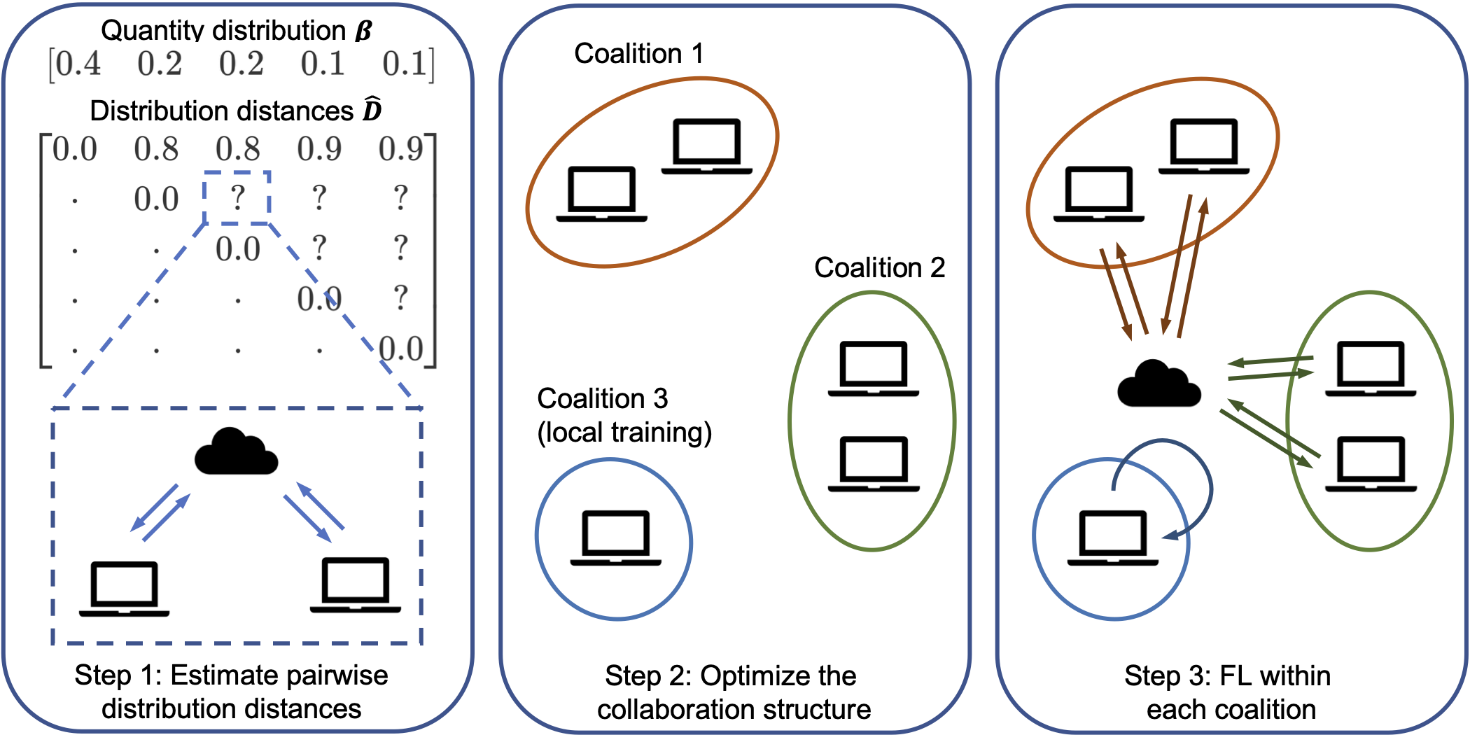
We propose FedCollab to alleviate the negative transfer problem in federated learning (FL) by clustering clients into non-overlapping coalitions based on their distribution distances and data quantities.
- Theory: We analyze how clustered FL performance is affected by two key factors: distribution distance and data quantity.
- Algorithm: We propose FedCollab to solve for the best collaboration structure.
- Extensive experiments: We test FedCollab under label shift, feature shift and concept shift with various models / datasets.
Background

In global FL, multiple clients collaborate to train a shared machine learning model without sharing their raw data. Although global FL can utilize more data samples, when clients have non-IID data, global FL suffers from the negative transfer problem, i.e., the global model can be even worse the local model.
Clustered FL groups clients into coalitions based on distributions; each client only shares model with clients in the same coalition.
Question: What is the optimal clustering structure, i.e., which clients should train shared model?
Theoretical Analysis
We consider an FL system with \(N\) clients, each client \(i\) has \(m_i\) samples \(\hat{\mathcal{D}}_i = \{(\boldsymbol{x}_k^{(i)}, \boldsymbol{y}_k^{(i)})\}_{k=1}^{m_i}\) i.i.d. drawn from its local distribution \(\mathcal{D}_i\). \(h\) is the ML model and \(\ell\) is the risk function. Denote the quantity distribution \(\boldsymbol{\beta} = [\beta_1, \cdots, \beta_N] = [\frac{m_1}{m}, \cdots, \frac{m_N}{m}]\) where \(m = \sum_{i=1}^N m_i\).
- Client \(i\)’s local empirical risk: \(\hat{\epsilon}_i(h) = \frac{1}{m_i}\sum_{k=1}^{m_i} \ell(h(\boldsymbol{x}_k^{(i)}), \boldsymbol{y}_k^{(i)})\)
- Client \(i\)’s local expected risk: \(\epsilon_i(h) = \mathbb{E}_{(\boldsymbol{x}, \boldsymbol{y}) \in \mathcal{D}_i} \ell(h(\boldsymbol{x}), \boldsymbol{y})\)
Theorem 3.3. (informal) Let \(\hat{h}_{\boldsymbol{\alpha}_i} = \text{argmin}_{h \in \mathcal{H}} \sum_{j=1}^N \alpha_{ij} \hat{\epsilon}_j(h)\) where \(\sum_{j=1}^N \alpha_{ij} = 1\). With probability at least \(1 - 2\delta\),
\[\epsilon_i(\hat{h}_{\boldsymbol{\alpha}_i}) \leq \underbrace{\vphantom{\frac ab}\epsilon_i( h_i^* )}_{\text{irreducible error}} + \ 2 \underbrace{\vphantom{\frac ab}\phi_{|\mathcal{H}|}(\boldsymbol{\alpha}_i, \boldsymbol{\beta}, m, \delta)}_{\text{quantity-aware function}} + \ 2 \sum_{j \neq i} \alpha_{ij} \underbrace{\vphantom{\frac ab}D(\mathcal{D}_i, \mathcal{D}_j)}_{\text{distribution distance}}\]where
- the quantity-aware function
- the distribution distance
Theorem 3.3 above shows that the error upper bound is controlled by (1) collaboration structure, (2) pairwise distribution distances, and (3) data quantities. Therefore, the optimal collaboration structure (that minimizes the error bound) depends on distribution distances and data quantities.

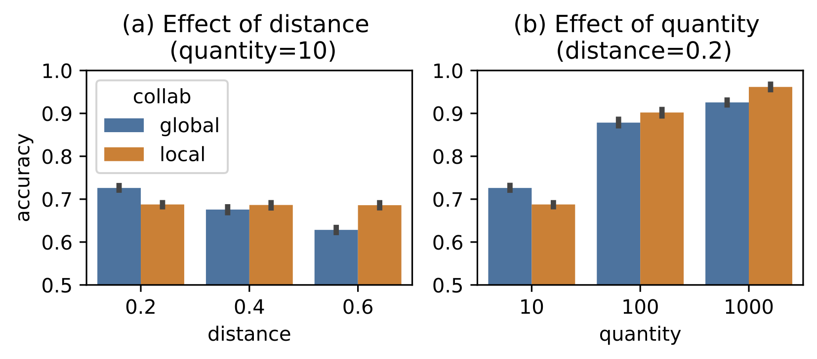
We consider an FL system with 2 clients, each has the same number of samples.
- Clients prefer collaborators with smaller distribution distances. In Figure 2(a), the collaboration is only beneficial when distribution distance is small enough.
- Clients with more data are pickier in the choice of collaborators. In Figure 2(b), the collaboration is only beneficial when quantity is small.
Algorithm: FedCollab
FedCollab solves the collaboration structure bv minimizina an empirical estimation of the error bound in Theorem 3.3.

Step 1: Estimate pairwise distribution distance. Train a client discriminator \(f: \mathcal{X} \times \mathcal{Y} \to \{0, 1\}\) for each pair of clients with FL algorithm. \(\lvert123\rvert\).
\[\hat{D}_{ij} = 2 \cdot \text{BalancedAccuracy}(f, \{\hat{\mathcal{D}}_i^{\text{valid}}, 1\} \cup \{\hat{\mathcal{D}}_j^{\text{valid}}, 0\}) - 1\]- When \(\mathcal{D}_i, \mathcal{D}_j\) are distinctly different, balanced accuracy \(\approx 100\%\) and \(\hat{D}_{ij} \approx 1\).
- When \(\mathcal{D}_i, \mathcal{D}_j\) are similar, the classifier cannot outperform random guessing whose balanced accuracy \(\approx 50\%\) and \(\hat{D}_{ij} \approx 0\).
Step 2: Optimizethe collaboration structure. Minimize the sum of empirical error upper bounds with greedy method.
\[\mathcal{L}(\boldsymbol{A}, \boldsymbol{\beta}, m, \hat{\boldsymbol{D}}) = \sum_{i=1}^N \left( \frac{C}{\sqrt{m}} \sqrt{\sum_{j=1}^N \frac{\alpha_{ij}^2}{\beta_j}} + \sum_{j=1}^N \alpha_{ij} \hat{D}_{ij} \right)\]where \(C\) is a hyperparameter and the collaboration structure
\[\boldsymbol{A}_{ij} = \alpha_{ij} = \begin{cases} \frac{\beta_j}{\sum_{l \in \mathcal{C}_k} \beta_l}, & \text{if } i \in \mathcal{C}_k, j \in \mathcal{C}_k, \exists \text{ coalition } k \\ 0, & \text{otherwise} \end{cases}\]Step 3: FL within each coalition. Notice that since the collaboration structure and the FL model are optimized independently, FedCollab can be seamlessly integrated with any GFL or PFL algorithms in this stage.
Experiments
Setup. We consider 20 clients with unlabanced data quantities \(\beta_0 = \cdots = \beta_9 \gg \beta_{10} = \cdots = \beta_{19}\). We consider three kinds of distribution shifts: label shift, feature shift and concept shift.
- Label shift: each client has different label distribution.
- Feature shift: each client’s image is rotated at different angles.
- Concept shift: each client’s label is permuted.

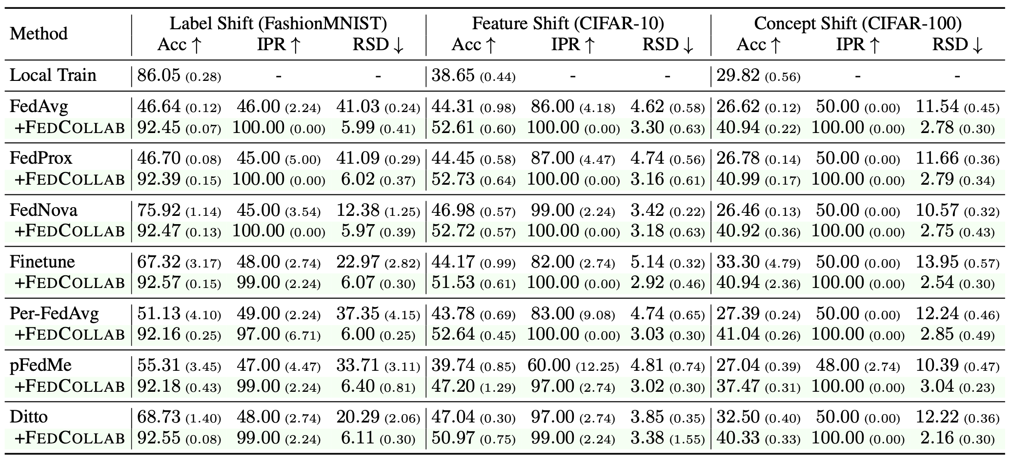
FedCollab alleviates negative transfer for both global FL and personalized FL

- IPR - % of clients with \(\epsilon_i(\hat{h}_{\boldsymbol{\alpha}_i}) < \epsilon_i(\hat{h}_{i})\), i.e., FL model is better than local model
- RSD - standard deviation of \(\{ \epsilon_i(\hat{h}_{i}) - \epsilon_i(\hat{h}_{\boldsymbol{\alpha}_i}) \}_{i=1}^N\), i.e., whether clients have uniform accuracy gains
FedCollab outperforms previous clustered FL algorithms

- FedCollab explicitly uses the quantity distribution during collaboration optimization.
- FedCollab estimates high quality distribution distances.

Citation
If you find this paper helpful to your research, please consider citing our paper:
@InProceedings{bao23b,
  title = 	 {Optimizing the Collaboration Structure in Cross-Silo Federated Learning},
  author =       {Bao, Wenxuan and Wang, Haohan and Wu, Jun and He, Jingrui},
  booktitle = 	 {Proceedings of the 40th International Conference on Machine Learning},
  year = 	 {2023}
}